All models are wrong, but some are useful.
-- George E. P. Box
Does installing an antivirus that catches 2% more malware really make a difference? Should antiviruses try to concentrate on catching yet unknown malware requiring a small delay or is it acceptable if they primarily rely on simpler and faster signature-based detection? These and many other questions can be answered by modeling the behavior of malware and later mapping it to existing malware infection data.
In this post we will try to apply a modeling technique commonly used for epidemic and population modeling to predict the spread of malware. However, first we should go over a simple application of differential equations to model monthly fluctuations in populations of foxes and rabbits, because although the application is very different, the equations are not.
Foxes and Rabbits

First, let’s establish what we are trying to model. We are interested in figuring out how the populations of foxes and rabbits fluctuate over time. We know that rabbits would multiply exponentially if there were no predators. We know that for foxes to grow and flourish there need to be some rabbits around as they are the food source. We also know that both foxes and rabbits can die of old age. There are many other things that are true about foxes and rabbits, but let’s say that these are the main contributors to the population dynamics.
Luckily for us, there already exists a pair of equations that can be used to model just this scenario. They are called Lotka-Volterra equations and different variations of these equations are used in ecology and epidemiology to model animal population dynamics and disease proliferation.
Without further ado, the equations are below:
In the first part, we see that \(dx/dt\), or change in \(x\) (the rabbit population) over time, is assumed to grow (\(xa\)) unless subject to predation (\(-bxy\)) and rabbits dying of old age (\(-cx\)).
In the second part, we see that \(dy/dt\), or change of \(y\) (the fox population) over time is dictated by the rate of rabbit consumption (\(ebxy\)) and natural death of foxes over time (\(\delta y\)). A more detailed explanation is found on the equation wiki page.
Integrating these analytically can be daunting especially if there are more equations and variables. We'll use a simple numerical integration technique called Midpoint Method to integrate the equation numerically and actually observe these trends.
A future point depends only on the previous point. So the population of rabbits tomorrow can be estimated from knowing today's populations of both foxes and rabbits.
In Python, to calculate \(x_{t+1}\) and \(y_{t+1}\) for each day \(t\) in \(\{0..730\}\), we can do the following:
import numpy as np
import pylab as pl

def calc_lv(x, y, coefs):
    x_new = x * (coefs['a'] - coefs['b'] * y - coefs['c'])
    y_new = y * (coefs['e'] * coefs['b'] * x - coefs['d'])
    return x_new, y_new

def midpoint_method_lotka(t, x, y, coefs, dt, N):
    for i in range(N):
        dx1, dy1 = calc_lv(x[i], y[i], coefs)
        dx2, dy2 = calc_lv(x[i] + dt * dx1 / 2, y[i] + dt * dy1 / 2, coefs)
        x[i + 1] = x[i] + dt * dx2
        y[i + 1] = y[i] + dt * dy2
        t[i + 1] = i * dt
    return t, x, y

def do_lotka():
    a = 0.04
    b = 0.0005
    c = 0.0001
    d = 0.2
    e = 0.1
    dt = 0.01
    days = 730
    N = int(days / dt)
    coefs = {'a': a, 'b': b, 'c': c, 'd': d, 'e': e}
    x, y, t = np.zeros((3, N + 1))
    x[0] = 200  # Initial prey data
    y[0] = 50   # Initial predator data
    t, x, y = midpoint_method_lotka(t, x, y, coefs, dt, N)
    pl.plot(t, x/10, 'g', t, y, 'r')
    pl.show()
Implementing it in JavaScript results in the following graph where you can play with the coefficients:
From the plots you can see that the populations are oscillating. The foxes die off when there are no rabbits. Since there are fewer foxes, rabbits’ population increases. As soon as the rabbit population starts increasing, the fox population also starts increasing. A larger number of foxes eats rabbits faster than they multiply, so rabbit population drops and the cycle continues.
This demonstrates that if we know (or make assumptions about) some rules of interaction between distinct populations, then we can write down some differential equations and analyze the dynamics of these populations.
Onto Malware
To model the spread of malware, we will use the same paradigm but design it a little differently to reflect the nature of malware proliferation. Specifically, we will simply use our knowledge of how malware can spread to design equations that allow us to model and analyze the dynamics of its proliferation.
We are going to model a network of computers that periodically talk to each other. The network can be a TCP/IP network or just some computers that share information via USB drives.
Vulnerable computers can be infected with 2 types of malware – known malware and so-called 0-Day malware. The distinction here is that AV companies have signatures for known malware.
Once a computer is infected and that infection is detected, it can be quarantined. Here quarantined means that a sysadmin has isolated it from the rest of the network. After the computer is quarantined it is disinfected and then put back on the network.
Antivirus companies periodically update their signatures, so computers infected with unidentified malware eventually get converted to an infection with identified known malware, i.e. malware they were infected with can become “known”. Malware writers are more likely to write malware if there are a large number of known-vulnerable computers and some number of active malware already in the wild. This way the effect of each malware would be amplified and they could improve upon extant malware.
Malware periodically stops working and bad domain/IP lists are periodically updated to block C&C server traffic. 0-Day malware is harder to write, but it is probably written better and has a higher chance of succeeding.
We can express these ideas with differential equations. One way to do it is the following:
- \(V\) or the Vulnerable population is the normal population of computers within a network that have a potential to get malware.
- \(Q\) or the Quarantined population are the computers that have been quarantined after a sysadmin found some malware on the machine and decided to take it off the network so that it doesn’t infect other computers.
- \(I\) or the Computers Infected with malware.
- \(U\) or the Computers infected with Unidentified malware/0-Days.
- \(W\) or the regular Worm/Malware C&C server population is the number of known malware in the wild.
- \(Z\) or the 0-Day Worm/Malware C&C population.
The coefficients mean the following:
\(c\) and \(\epsilon\) are the probabilities that a given known malware and 0-Day malware, respectively, would be functional and not immediately detected.
\(a\) and \(a_0\) are the coefficients of expected infected computers where \(aW\) and \(a_0 Z\) are the expected number of new infected computers for regular malware and 0-Days, respectively.
\(f\) is the catch rate of known malware when it already exists on a machine.
\(h\) is the fraction of unknown malware that is discovered and labeled as malware by AV companies every day.
\(b\) is the fraction of quarantined computers that become disinfected and go back on the network. This is really the response time of a SysAdmin/IT forensics in dealing with known infections.
\(g\) is the catch rate of unknown malware. This is in the same role as \(f\), but here no signatures exist.
\(k\) is the clustering coefficient for computers. That is, within a set of computers that share information among themselves, it is possible that there are clusters of computers that are more connected (e.g.: sharing USB drives).
\(l\) and \(n\) are the coefficients of malware and 0-Day malware growth.
\(m\) and \(o\) are the coeffients for reduction in number of C&C servers. These could either represent malware no longer working because it is not compatible with system updates or C&C servers getting blacklisted.
\(p\) and \(p_0\) are the coefficients of expected number of C&C servers where \(pW\) and \(p_0Z\) are the expected number of new C&C servers for regular malware and 0-Days, respectively.
Note: \(e^{-aW}\) represents the fraction of computers not infected according to a Poisson distribution with a value of \(0\). That is, \(\frac{\lambda^k e^{-\lambda}}{k!}\) where \(k=0\) and \(\lambda=a\). Since there are \(W\) malware in the wild, the equation becomes \(e^{-a^W}\) or \(e^{-aW}\). Therefore \(1-e^{-aW}\) represents the fraction that is infected. \(aW\) then represents the Poisson parameter of expected number of computers infected per day. We use a Poisson distribution here because it can be used to predict frequencies of occurrences of rare events.
This version of the model assumes the following:
- Infected computers cannot infect others directly.
- All vulnerable computers are equally likely to be infected.
- There is only one infection per computer.
- Probabilities of infection are given by a Poisson distribution.
- One malware entity per C&C server.
- Total number of computers remains the same.
To integrate these numerically, we will use midpoint method again. You can find the python implementation for that here. It is also implemented/plotted below in JS, so you can play with the coefficients of the malware diagram here:
Meaning and Implications
To figure out what the model implies and represents we will set some coefficients to zero or 1.
Setting \(c\) and \(l\) to zero removes the effects of known malware, while setting \(\epsilon\) and \(n\) to zero removes the effects of 0-Days.
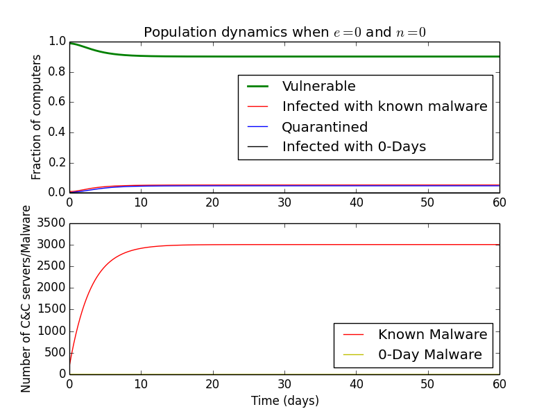
If we set \(b\) to zero, this could represent a very lazy IT department that never fixes infected quarantined computers.
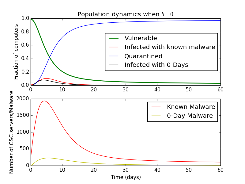 On the other hand, setting \(b\) to \(1\), can represent a very active IT department that fixes all infected computers within a day.
If we set \(f\) and \(g\) to \(1\), we have a situation where all malware is detected after just one day of being in the wild.
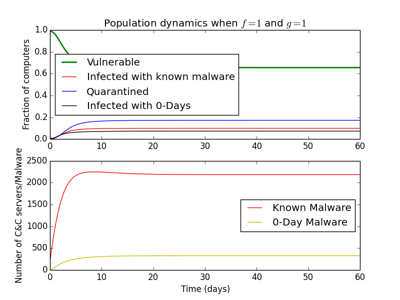
This could be a future sandbox that takes some time to reach its conclusion, but always finds the malware. Finally, if we set \(f\) and/or \(g\) to zero, this would represent an incompetent antivirus/sandbox that never detects anything if it gets past the initial defenses.
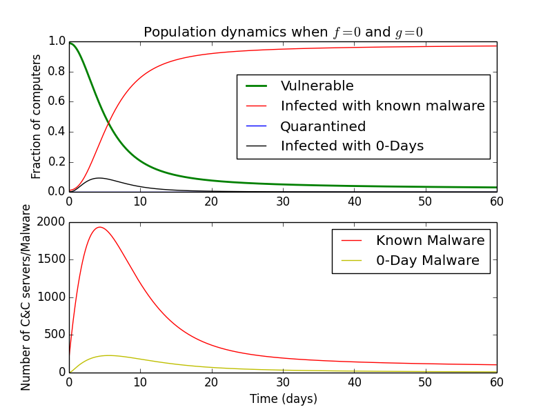
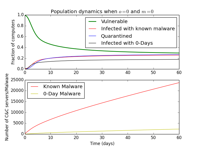
Since \(o\) and \(m\) are rates of malware C&C servers being blocked, setting them to zero results in unabated malware growth.
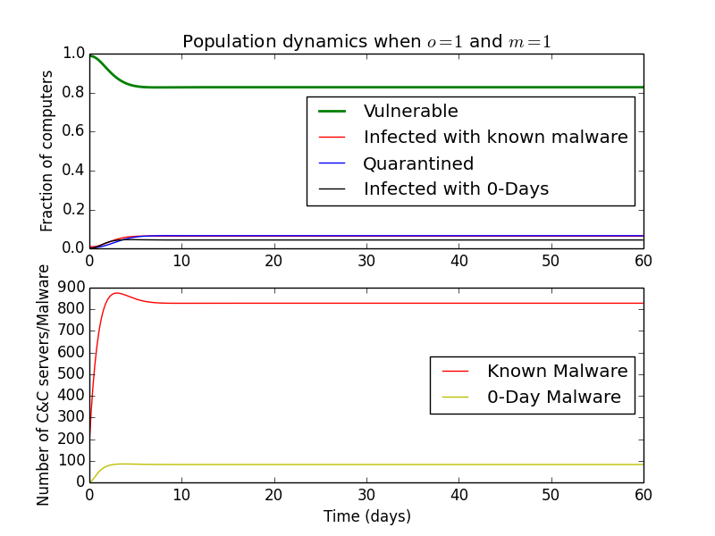
 At the opposite end of the spectrum, setting them to \(1\) might represent very active Domain/IP blocking where C&C servers disappear within a day after being active.
Without 0-Days
If we set \(\epsilon\) and \(n\) to zero, we are ignoring the effect of 0-Day malware and associated C&C servers. Thus we are left with
Here, \(c\) can be viewed as a coefficient that represents the fraction of malware that is not detected every day. Therefore, \(0\) corresponds to
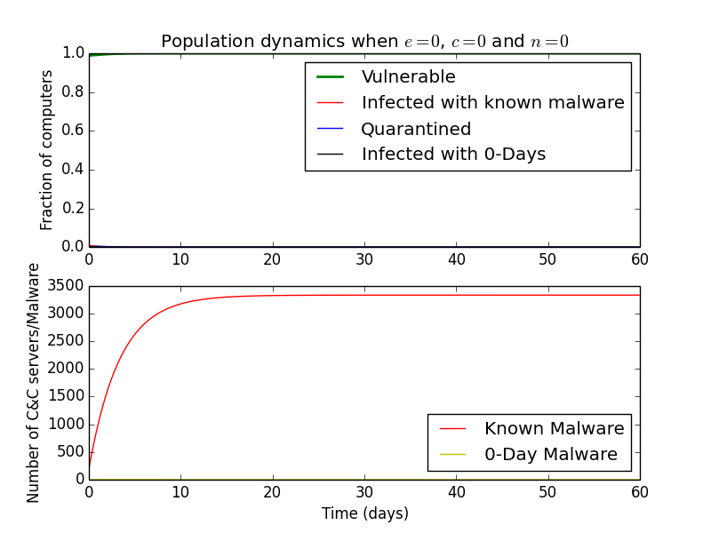 and \(1\) corresponds to malware not getting detected initially.
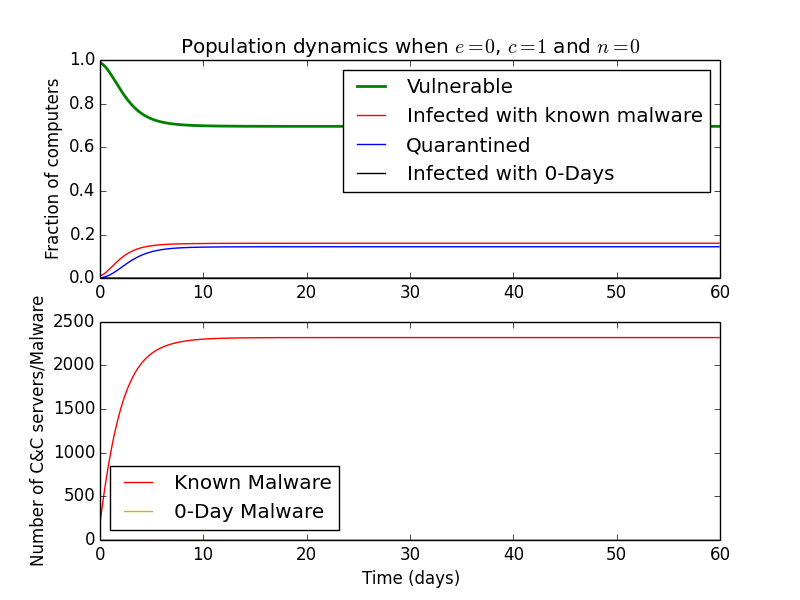 Setting \(c\) to \(1\), and \(f\) to \(1\) and leaving the rest of the coefficients at default values, we can see that some computers are still infected.
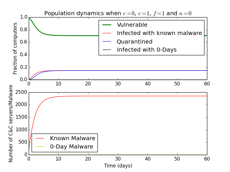
What this implies is that the malware gets on some computers and is wiped within a day. We are still left with a constant ≈\(10\%\) portion of computers being infected. However, if \(90\%\) of the malware that gets on is initially detected (\(c=0.1\)), only \(3\%\) of the computers are infected. Therefore, we can gather than initial detection plays a major role in reducing the number of infections.
Keeping \(f=1\) i.e. the detection after \(1\) day at \(100\%\), we can also answer whether it matters if an antivirus detects \(90\%\) or \(99\%\) of malware immediately. At \(90\%\) detection, \(2\%\) of computers are perpetually infected
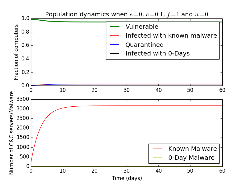 while at \(99\%\), none are.
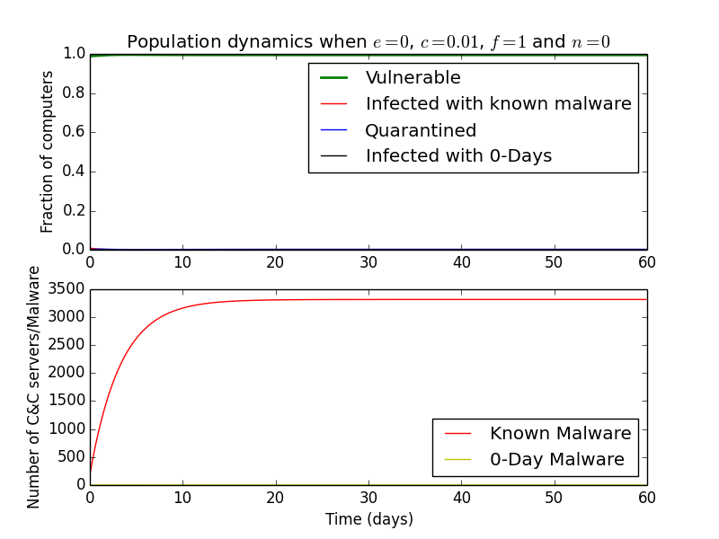 So in a world where all malware is known and if an antivirus can tell after a day if a computer is infected, it is indeed better to use an antivirus that detects \(99\%\) than \(90\%\) of the malware immediately.
Adding 0-Days
After setting \(\epsilon\) and \(n\) back to their original values, we can explore what happens to the system when we have 0-Day malware and C&C servers and how 0-Day detection affects the number of infected computers.
First, we can look at the effects of \(o\), the coefficient of detection of C&C servers. Increasing it surprisingly results in an increase in the number of active known C&C servers, but decreases in infected and 0-Day infected computers. This makes sense, because there are more vulnerable computers, so malware authors may be more likely to spread existing malware.
A similar effect can be observed if we increase the detection rate of 0-Day malware (\(g\)) or lower the fraction of working 0-Days (\(\epsilon\)).
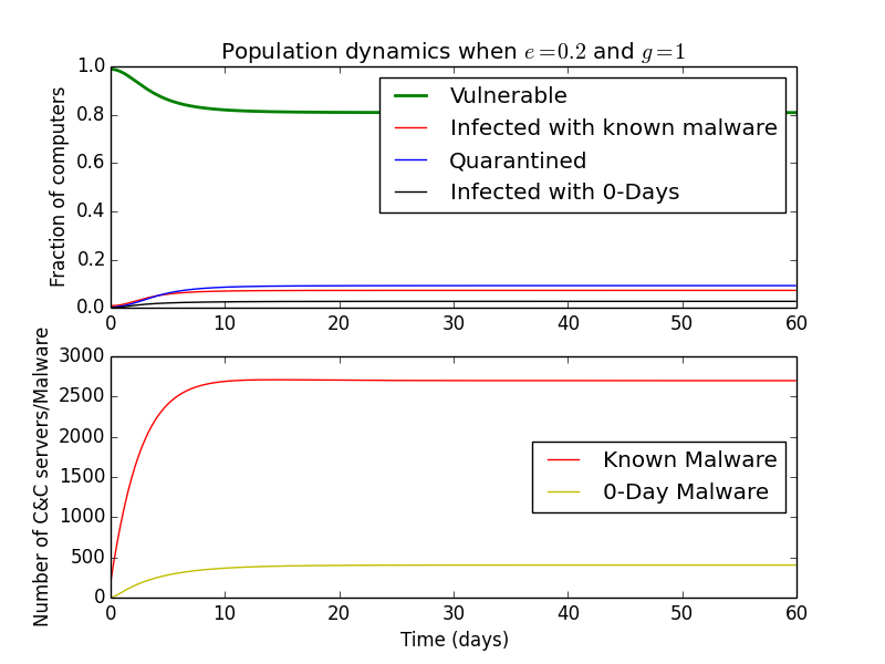 The number of C&Cs that control 0-Day and known malware increases, but the number of computers infected with either decreases.
Lessons learned
Although when creating the model we made a number of assumptions that may not always be true, these results can still be useful, especially if the model is fit to real data.
Small improvements in detection rate of known and 0-Day malware can make a big difference in the number of users subject to infection. For example, a \(9\%\) increase in the immediate detection can result in almost complete abolition of infected computer population, substantially decreasing the need for forensic analysis and potentially reducing required IT budget. Overall, quicker signature generation (increasing the \(f\) coefficient) and utilizing sandboxing techniques (increasing \(g\) and decreasing \(\epsilon\)) to detect 0-Days can have a profound impact in reducing the number of infected computers, thereby protecting users' data and preventing proliferation of botnets.
Full version of the Python model implementation can be found on Github.